Hierarchical Quadratic Programming for Robot Control
July 31, 2025
Quadratic Programming (QP)
Subset of Convex Programming.
Both efficient to solve and descriptive.
\[ \begin{align} & \min_x \; && x^T Q x + p^T x \\ & \text{s.t.} \; && A x = b \\ & && C x \leq d \end{align} \]
Problem 🤕
Problem: solve a set of tasks that cannot be satisfied concurrently.
E.g., maintain an end-effector pose (task), avoid obstacles (safety), and minimize energy consumption (efficiency).

Solution Approaches
Techniques to deal with redundancy:
- Standard approach
- Singularity-robust approach
- Reverse priority approach
- Hierarchical Quadratic Programming (HQP)

Introduction
Research Goal: consider the contact compliance in the control design.
Contributions:
- The Soft Bilinear Inverted Pendulum (SBIP) model is proposed and used in the Motion Planner design.
- A Whole Body Controller is developed using Hierarchical Optimization and a soft contact model.
- The improvements granted by considering the softness in the MP and the WBC are evaluated.
- The proposed approach is tested in simulations and experiments.

Soft Bilinear Inverted Pendulum Model
Equations of motion of the SBIP model: \[ \begin{align} \ddot{x}_{CoM} &= \frac{g + \ddot{z}_{CoM}}{h_{CoM}} (x_{CoM} - x_{ZMP}) \\ \ddot{y}_{CoM} &= \frac{g + \ddot{z}_{CoM}}{h_{CoM}} (y_{CoM} - y_{ZMP}) \\ \ddot{z}_{CoM} &= - \ddot{\delta} = - g + 1/m (k_p \delta + k_d \dot{\delta}) \end{align} \]
Simplified model used to plan the base and feet trajectories over a long horizon.
The planner is a QP-based MPC that tracks a base velocity reference.

Tracking Controller
Full robot model used to plan over a short horizon with higher fidelity.
The equations of motion of a legged robot are \[ M(q) \ddot{q} + h(q, \dot{q}) = S^T \tau + J^T (q) f \] which can be split into the underactuated and actuated part as \[ \begin{align} M_a (q) \ddot{v} + h_a (q, v) &= \tau + J_a^T (q) f \\ M_u (q) \ddot{q} + h_u (q, v) &= J_u^T (q) f \end{align} \]
The optimization vector is \[ x_{opt} = \begin{bmatrix} \dot{v}^T & f^T & \delta_d^T \end{bmatrix}^T \]
From the optimization vector and the robot model, the joint torques are \[ \tau^* = M_a (q) \dot{v}^* + h_a (q, v) - J_a^T (q) f^* \]
| Priority | Tasks |
|---|---|
| 1 | Physical consistency |
| 2 | Actuation torque limits |
| Contact friction cone limits | |
| Force modulation | |
| 3 | Soft contact constraints |
| 4 | Base linear trajectory tracking |
| Base angular trajectory tracking | |
| Swing feet trajectory tracking | |
| 5 | Energy minimization |
| Contact forces minimization |
Comparison in Simulation
Four controller configurations compared using four KPIs and two different scenarios.

Problem
Actuators overheating during prolonged use.


Introduction
Research Goal: guarantee thermal safety and optimal performance using control.
Contributions:
- Consider the thermal dynamics in the control design.
- HQP based approach for constraints prioritization.
- Ablation study to evaluate the impact on performance.

Control Architecture
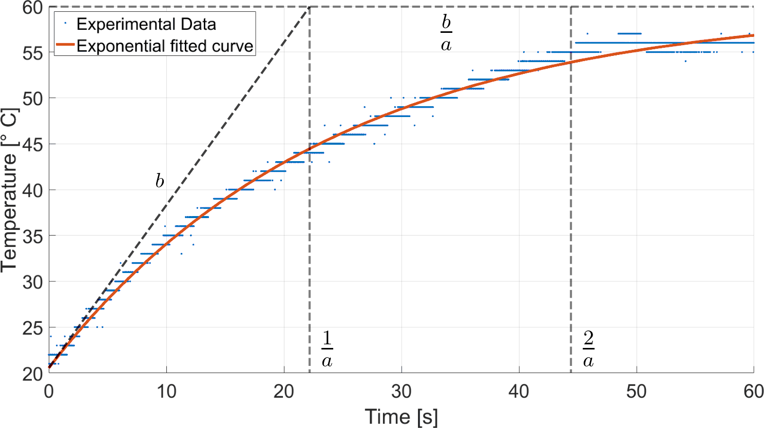
First order thermal model \[ \dot{T} = - \alpha (T - T_\text{amb}) + \beta | \tau | \]
Control Architecture

Optimization vector: \[ x = \begin{bmatrix} q^T & \dot{q}^T & T^T & \tau_s^T \end{bmatrix}^T \]
Tasks:
- Dynamic consistency, Thermal model, Epigraph reformulation
- Thermal safety, Safety limits
- Primary task (e.g., end-effector pose)
- Secondary tasks (e.g., control energy minimization)
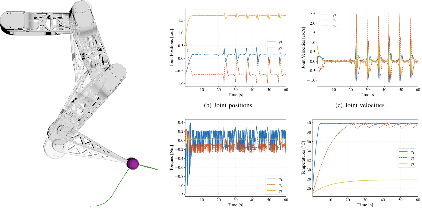
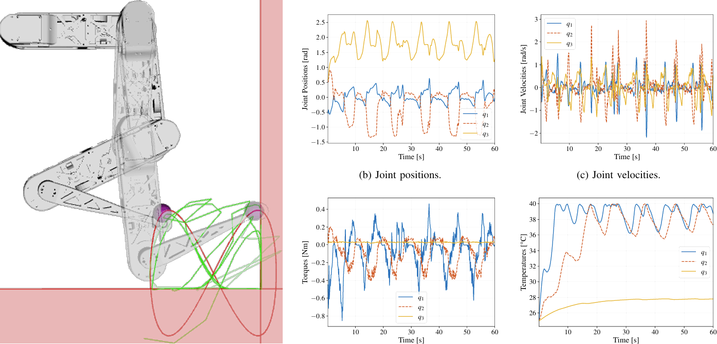
Results - Reach and Hold
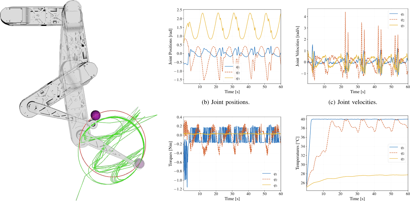
Results - Circle
Results - Lemniscate
Conclusion
- Considering the temerature dynamics in the control can avoid overdimensioning the hardware or downsizing the task.
- HQP effectively guarantees thermal safety.
- Other approaches (e.g., CBFs) can further enhance performance in certain scenarios.